bLUNA Liquidation Risks - Machine Learning Modelling
Explore the worst-case scenarios for liquidation on Anchor. When have the most liquidations occurred, how much, and how many users were impacted? Under what scenarios might significant liquidations occur again?
The data obtained from Flipsidecrypto contain 3 variables only; Time of data point collection, Liquidation amount in USD, and LUNA price.
Note that the data weren't collected regularly, in other words they weren't collected hourly or daily. In fact, the average difference between two successive periods in my data is 7.63 hours, and the median is 2 hours. The differences in periods were highly positively skewed. All my analysis should be interpreted as such.
I had to manually introduce some more new useful data using what I have, this was done as follows:
- I extracted LUNA price gains each period (i.e. LUNA_gains_t2 = LUNA price at t2 - LUNA price at t1).
- I made the liquidation categorical variable, marking what I termed Big Liquidations; these are liquidations with more than 1 million $ in value.
I then introduced new variables (let's call them dispersion indicators, I'll define them in the next paragraph);
- 9 rolling LUNA price standard deviation columns, with windows from 2 to 10 periods (rolling_sd_2, rolling_sd_3,.. etc.)
- 9 rolling Sortino ratio columns, with windows from 2 to 10 periods (rs_2, rs_3,.. etc.)
- 9 rolling Negative standard deviation columns, with windows from 2 to 10 periods (negative_sd_rolling_2, negative_sd_rolling_3,.. etc.)
The following principal component variables are ordered by explanatory importance (i.e. by their summarizing power):
-
Dim1: seemed to be trying to capture sign flips in standard deviation of LUNA price gains. In other words, it seemed concerned in knowing whether the price has gained or lost in comparison to previous periods. I propose calling it "price_direction". The higher this value, the more downside volatility exists, the less, the higher other dispersion indicators exist.
-
Dim2: It looked like this axis was trying to capture time periodicity. It had no negative values. For example, it was giving more weight to extended standard deviations (e.g. rolling Sortino 8), and less weight for short periods (i.e. rolling Sortino 2). Therefore I propose calling it "time_horizon". The higher this value, the more extended the time frame is, and vice versa.
-
Dim3: This dimension was hard to explain, but it seemed it was trying to capture—timewise—how extended is the risk of making gains (i.e. Sortino values). In other words, it gave the highest weight to rs_2 followed by rs_3, while the downside SD rolls were near zero. Its most negative value was rolling_sd_10, followed by rolling_sd_9. I propose calling it "risk_extension". The higher this value, the more narrow the time frame is and the more likely it is capturing Sortino ratio. The more negative this value, the more extended the time frame and the more likely it is capturing standard deviations proper.
-
Dim4: was more trying to capture proper and classic price action. The fact that the highest variable loading on this axis was LUNA gains supports this understanding, the next highest loading was rolling_2 standard deviation. Therefore I propose to call it "price_action".
The task I decided to pursue is not to perfectly know how much liquidations will happen. I chose a more conservative goal, the hypothesis is as follows:
- We can predict liquidations with more than coinflip-chance using data in hand before liquidations happen
At the beginning of the analysis, the data were split into a training set (85% of them), and a testing set (15%). It must be mentioned that the available data is scarce, and this imposes a challenge on the analyst. Had we possessed more data, the results would be cleaner.
All of the following results and analytics are calculated on the testing set.
I defined liquidations in two ways:
- A continuous manifestation: The raw amount of liquidations in USD.
- A categorical manifestation: I marked the "worst case scenarios", which I called Big Liquidations (whether they are more than 1 million $ or not). If a big liquidation took place at some period, I add a "1" to the row, otherwise "0" is added.
I did this because we want to know 2 information: whether we are about to hit a big risk period (a simple "YES" or "NO" can answer this, in machine learning terms; it is a classification task), and how much are we expecting liquidations to be in USD (of which the response should be an amount or quantity, or as it is called in machine learning statistical terms; a regression task).
I am going to model liquidations using pre-existing data, with machine learning techniques.
In a previous entry on flipsidecrypto, I explored bLUNA liquidations in time. I argued that the speed by which the price of LUNA falls at times of bear markets is a predictor of liquidations.
Let's retake a look to bLUNA liquidations in time, plotted against LUNA's price in the market. Liquidations are noted to be spikey and sudden.
Another interesting phenomenon was that liquidations were correlated with LUNA's price. I provided some speculations for the reasons behind this.
In this article, I am going to expand on my previous work, and see if liquidations are predictable.
I used R software, with special utilization of the caret library, which allows me to use my data into machine learning algorithms.
I used 5 methods for analysis: Linear Regression, Logistic Regression, KNN, Random Forests and Xgboost.
To do this, the following data were downloaded from Flipsidecrypto.
> If you only want to know the answer without reading through the statistical analysis behind my work, please skip to the conclusion part at the end.
In the aforementioned article, I introduced the concept Speed of Collapse (SoC), a quantity measuring how quickly the price is falling from a local maximum.
But SoC only dealt with downside changes in the price, it completely ignores price action when it is going up or sideways. We want a tool to deal with price and liquidations at all times, whether the change is downside or not.
Therefore, some new metrics had to be introduced, mainly ones dealing with volatility as we will explain later.
Why am I introducing many new variables? because I am motivated by hunch and suspicion that some or all of them contribute to predicting liquidations. I am going to experiment with them to find out which ones are relevant and which are not.
Therefore, another key takeaway from this article will be helping future analysts decide which techniques and variables are useful and which should be avoided to save time and effort.
Though these variables are not the same, they do contain a lot of redundancies, we can check this with correlation tests, which I did and resulted indeed in high values. Luckily, we can eliminate redundancies and summarize our variables while at the same time maintain the most utility with a statistical technique called Principal Component Analysis (PCA). I used the method Singular Value Decomposition in my analysis. This analysis will result in new variables called "principal components".
I was able to bring down 29 variables to 4 variables (or principal components) only while maintaining 91.55% of the variability in the data. The 29 variables were: all of my dispersion data, the LUNA price, and the LUNA gains. The 4 resulting principal components are totally uncorrelated.
If the data indeed contain redundancies, then my new PCA set should be more useful. If the preliminary data, as tautological as the variables might sound, contain unique information, then they should be more useful.
-
Rolling in statistics is synonymous to "moving", as in "moving average". It means that a certain time window is taken, and some statistical metric is applied to that window. All of my rolls had frames from 2 to 10 periods. For example, roll_2 took the current period's datum and the previous datum only, while roll_3 took the current datum and the previous 2 data points.
-
Standard Deviation (SD): is a famous dispersion statistic, it quantifies how far a value is from the variable's mean. So an SD of 1.5 means it is 1.5 units (or SDs) far from the average. It can be negative for values below the mean. A rolling standard deviation means that SD was calculated only for values within a certain time window.
-
Sortino ratio: it basically divides gains by the amount of downside deviation. This means that it gives us an indication of how much gain we are having against the risk and negative price fluctuations we are confronting. It helps answer the question "Is this gain worth the risk?". I use this metric to partially compensate me for Speed of Collapse. I was able to roll Sortino ratios with an ad-hoc function of my own.
-
Negative standard deviation (or downside deviation): It is the standard deviation of negative gains only. So this metric is mostly effective when the market is bearish. It is in the calculation of Sortino ratio, but I chose to include it because I want a metric that better captures my Speed of Collapse. Downside deviation is perfect for this, since it should conceptually and theoretically be a valid alternative for SoC. Thanks to basic algebra, I can calculate this by multiplying gains with the Sortino ratio.
After running all models for a couple of times, I gained an understanding of what is useful and what is not. I recognized that the PCA data is less useful, so I decided to only work on the preliminary full non-PCAed data.
To avoid flukes, I decided to run each model 10 times, with a new partitioning at each. The partitioning was made at random maintaining the ratio of 85% for training and 15% for testing. I would then report the average of my metrics and consequently confirm my guesses.
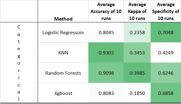
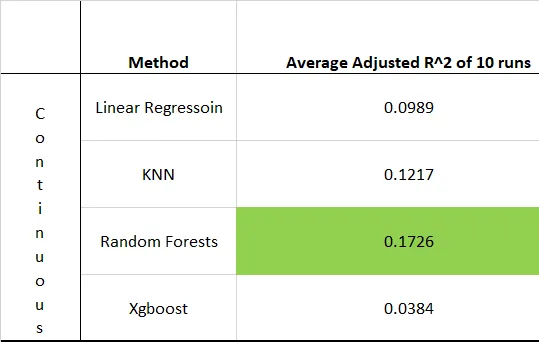
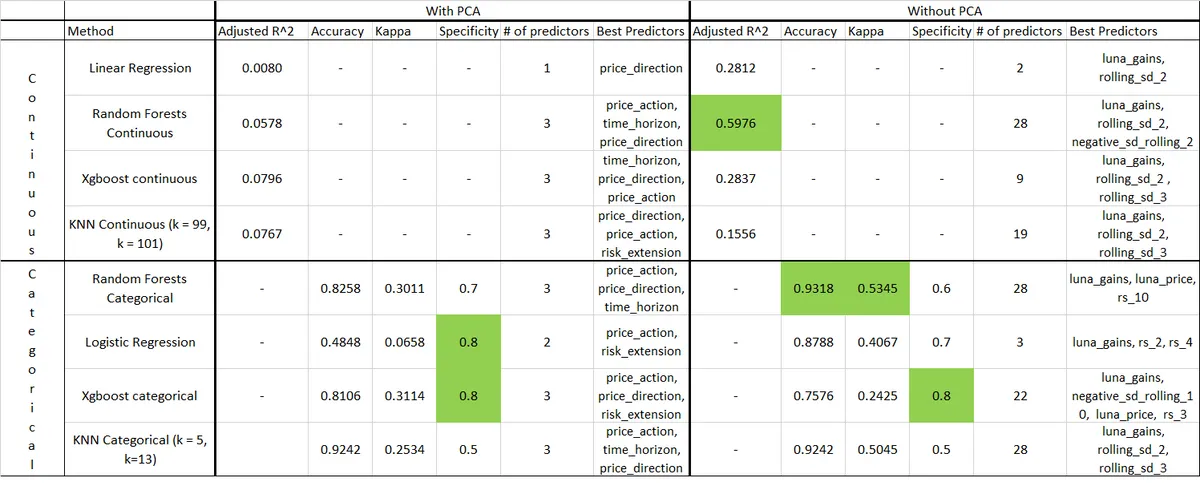
The results were as follows (I again highlighted the highest values in green shades).
These results are great, they indicate that we can predict liquidations with more-than-flipcoin chance. But some numbers seemed suspiciously high for me (too good to be true). I suspected they might be flukes, probably because of the models' sensitivity towards data partitioning (i.e. into testing and training groups, which might had been partitioned into some weird distributions). Therefore, I proceeded for further optimization.
I marked the highest metric in green to draw attention to the method. And for those who are interested in sparsity, I also showed how many variables each model is using (stepwise method was used when applicable). I showed in another column the most important variables utilized by the model to make its predictions.
For measuring the continuous USD liquidations variable, the only metric of interest I mention is R-squared. It indicates how much of the variance in USD liquidations is predicted by the model. An R^2 of 1 means the model is perfectly able to predict the variable of interest. The Random Forests model was able to predict a whooping 59.76% of liquidation amounts. This is considered relatively good, indeed, very good.
As for the categorical Big Liquidations variable, I mention 3 metrics: accuracy, kappa and specificity.
Kappa is my most important classification metric, it tells us how much better than coin-flip our model is. A kappa of 1 means that the model is perfect, while that of 0 means you are coin-flipping. A Kappa of -infinity means the model is doing the complete opposite of what it is supposed to do. A Kappa between 0.4 and 0.6 is taken to be fairly good. (e.g. 0.5 means we are 50% better than flip-coin).
The next important bit comes from specificity: the amount of Big Liquidation predictions that the model was successfully able to predict. (e.g. 0.5 means we were able to successfully predict 50% of Big Liquidations)
The least important of the three is accuracy, which is the amount of correct predictions out of all predictions. This metric is notoriously misleading since most of the data is highly skewed, causing sometimes classifiers that answer with all NOs (or all YESs) to have high accuracies. (e.g. accuracy of 0.9, means 90% of the data were classified correctly).
The highest Kappa was for my Random Forests classifier. It also had the highest accuracy. While the highest specificity was won by the Xgboost classifier.
I can now comfortably say that we are able to predict liquidations.
I, by subjectively assessing these results, tend to prefer choosing Random Forest algorithm for both the classification and the regression tasks; for predicting both the amount of possible liquidations, and whether we are about to enter a big liquidation risk period.
Random Forest (RF) algorithm has brought acceptable results. These numbers might not seem too attractive for some, but with the scarce data available in hand, and lack of wide scope of variables, I think these results should be appreciated.
Again, the aim of this article is not sniper accuracy, but merely to make sure that "liquidations" are predictable.
We can note that the continuous regression model was more so utilizing short-term price action, while the categorical classification task was more utilizing medium to relatively longer term risk indicators. Many readings for the same model can be made, but this is my personal view.
Utilizing the power of Machine Learning, in particular Random Forests algorithm, we can conclude that:
- liquidation amounts and risk of big liquidations can be predicted.
The main variables that allow us to do this are (please refer to the Definitions section for further explanation about these variables):
-
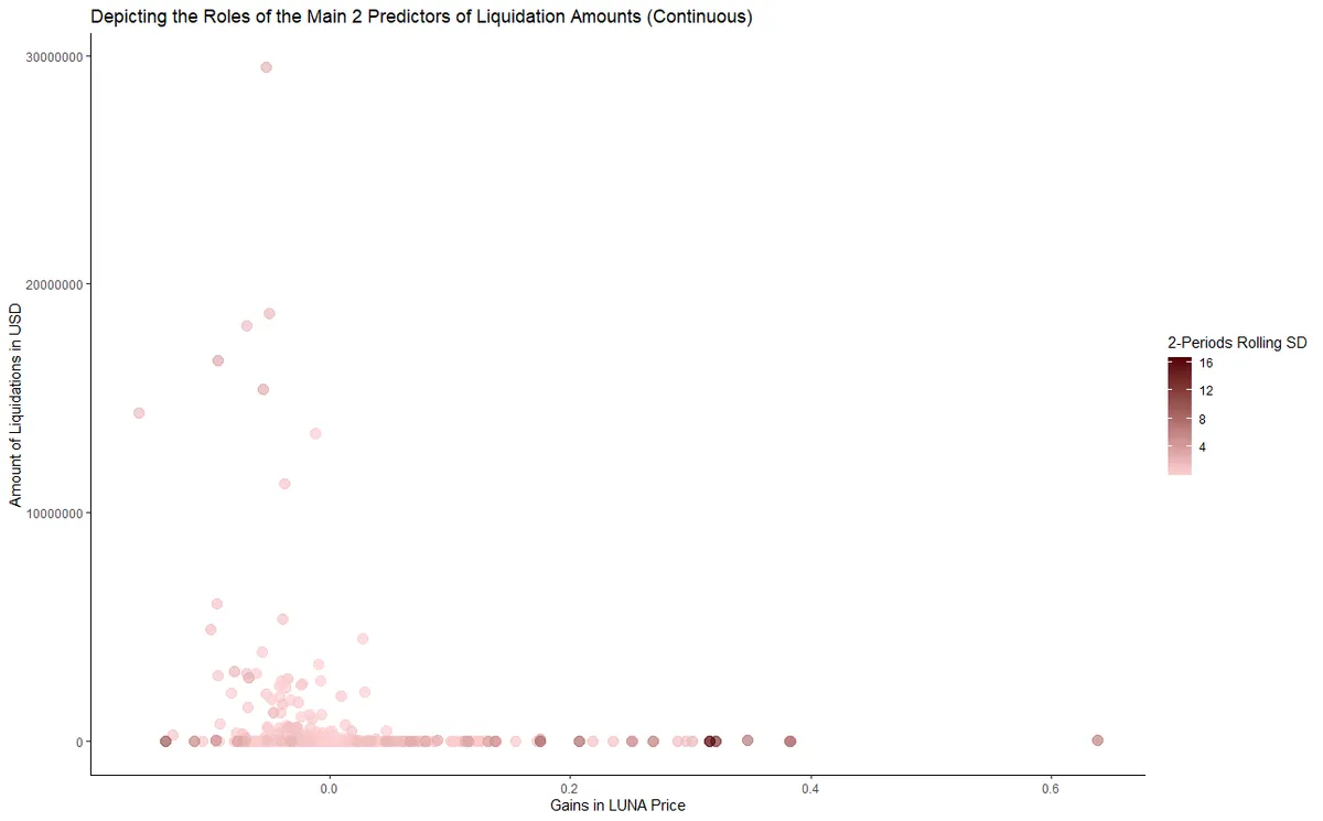
For continuous "Liquidation amounts in USD": LUNA price gains, rolling standard deviation for 2 periods of LUNA price, and rolling downside standard deviation for 2 periods of LUNA. Liquidation amounts are likely to become higher when; LUNA price gains are more negative, rolling_sd_2 is more positive, and negative_sd_rolling_2 is more negative.
-
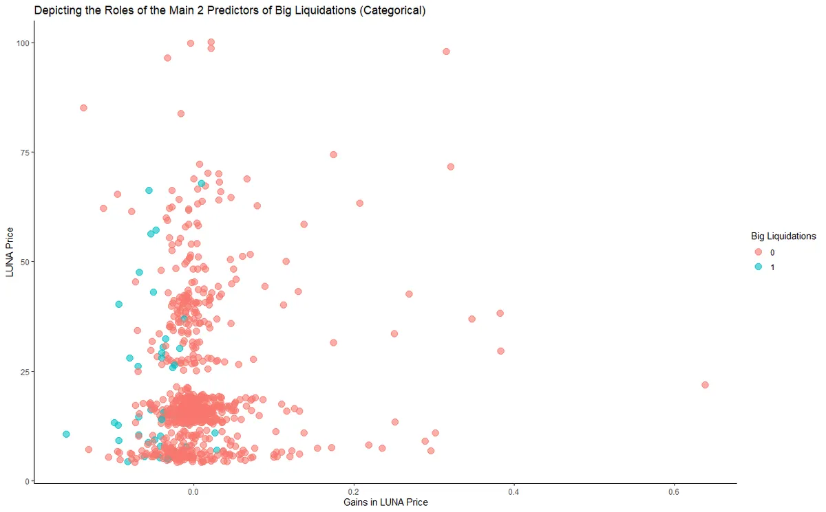
For categorical "Big Liquidation risk (liquidations > 1,000,000 $)": LUNA price gains, LUNA price proper, and rolling Sortino for 10 periods of LUNA. Though the RF algorithm is considered a black box, we can speculate—using correlation tests—that Big Liquidations become more likely when; LUNA price gains are more negative, LUNA price proper is higher, and the rolling_10 Sortino is more positive.
-
It is not worth it to summarize variables using PCA. The best predicting algorithm used nearly all variables mentioned in the Variables section above.
-
Rolling Standard Deviation, Rolling Sortino ratio, and rolling downside Standard Deviation all with windows from 2 to 10, in addition to LUNA price and LUNA price gains, a total of 29 variables, were nearly all used in the model predicting liquidations.
Trying to visualize the relationship is a bit abstract. Here is how the main two predictor variables from the RF models look like if plotted in the same chart with Liquidations. No clear cut criteria catches the eye (aside of the intuitive negative gains in LUNA price).
